Temporal Land Cover Change Detection Using AlphaEarth Satellite Embeddings
Table of Contents
This article was automatically translated from Japanese by AI.
Overview
In the previous article, I explored structure search using approximate nearest neighbor search with AlphaEarth Foundations Satellite Embeddings (AEF).
Satellite Embeddings are generated by a model trained on Sentinel-2 and Landsat optical imagery as inputs, with land cover classification data such as the USDA Cropland Data Layer as training targets. These Satellite Embeddings have been updated annually since 2017. This means that by comparing embeddings of the same location across different years, we can quantitatively assess how much the land cover has changed. Locations where large-scale land preparation from construction, farmland conversion, or new solar power installations have occurred should show changes in their year-over-year embeddings.
In this article, I leveraged this property to implement a system that detects land cover changes across all of Hokkaido between 2024 and 2025.
Change Detection from Satellite Imagery
Change Detection from satellite imagery is a technique that identifies surface changes by comparing satellite data from different time periods at a given location.
Two Approaches to Change Detection
There are broadly two approaches to change detection. The first uses visible/multispectral images directly, including pixel value differencing, vegetation index (NDVI, etc.) comparison, and deep learning-based change mask prediction. While highly interpretable due to being based on physical quantities, it suffers from false changes caused by differences in imaging conditions such as atmospheric conditions, solar elevation angle, clouds, and seasonal vegetation cycles. The second approach compresses images into embeddings using foundation models and then compares them. It obtains embeddings of the same location at different time periods and quantifies the magnitude of change using distance metrics such as cosine similarity. While it can capture semantic changes that are robust to imaging condition noise, interpreting “what changed and how” is difficult, and results heavily depend on the training characteristics of the embedding generation model.
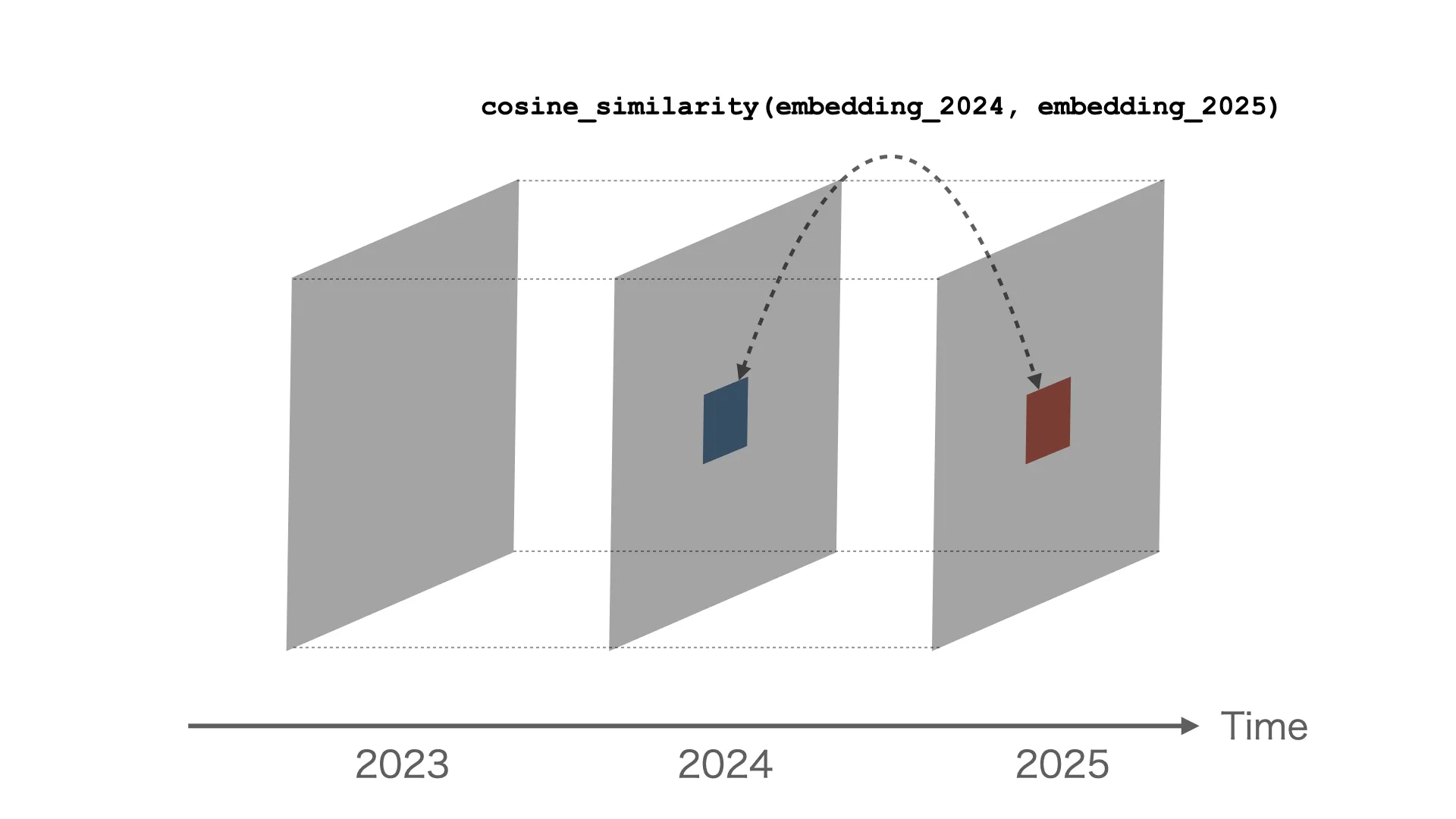
Comparing Embeddings via Cosine Similarity
For change detection in this study, I use cosine similarity between embeddings from two time periods using the Satellite Embeddings provided by AEF. Since AEF embeddings are unit vectors constrained to a unit hypersphere, cosine similarity equals the dot product of the vectors. Google Earth Engine’s similarity search tutorial also introduces similarity comparison using embedding dot products.
This works for annual comparison because AEF’s embedding space is consistent across years. The data catalog states:
The embedding space is consistent across years, and embeddings from different years can be used for condition change detection by considering the dot product or angle between two embedding vectors.
It is precisely because the 2024 and 2025 embeddings are placed in the same vector space that cross-year dot product comparisons are meaningful.
Incidentally, besides cosine distance, Euclidean distance and KL divergence are also used in embedding-based change detection. RaVÆn (Ruzicka et al., Nature Scientific Reports 2022) compared these metrics on VAE-based 128-dimensional embeddings and reported that cosine distance achieved the highest detection performance.
Method
Change Score Definition
I define a change score for any given location using cosine similarity.
change_score = 1.0 - cosine_similarity(embedding_2024, embedding_2025)
The change score ranges from 0 (no change) to a maximum of 2 (opposite vectors), but in practice, even locations with significant changes typically fall within the 0.3–0.9 range.
Data and Implementation
As in the previous article, I retrieved the 2024/2025 Satellite Embeddings for all of Hokkaido (139.3°E–145.9°E, 41.3°N–45.6°N) at 100m/pixel scale from the Earth Engine API. Each year’s data consists of approximately 15.66 million points with 64-dimensional vectors.
I also implemented connected component clustering using Union-Find to recognize spatially adjacent high-change points as contiguous regions. Cells with change scores exceeding a threshold (0.3) are connected via 4-connectivity on the grid, and for each connected component, I aggregate the cell count, mean change score, maximum change score, and bounding box.
Results
Overall Statistics and Trends
The change score statistics for all of Hokkaido from 2024 to 2025 are as follows:
| Metric | Value |
|---|---|
| Total points | 15,662,989 |
| Mean similarity | 0.9710 |
| Mean change score | 0.0290 |
| Maximum change score | 0.8842 |
| Points with change score > 0.3 | 111,040 (0.7%) |
The majority of points show high similarity around 0.97, indicating almost no change over one year. Only 0.7% of all points—approximately 110,000—exceed a change score of 0.3.
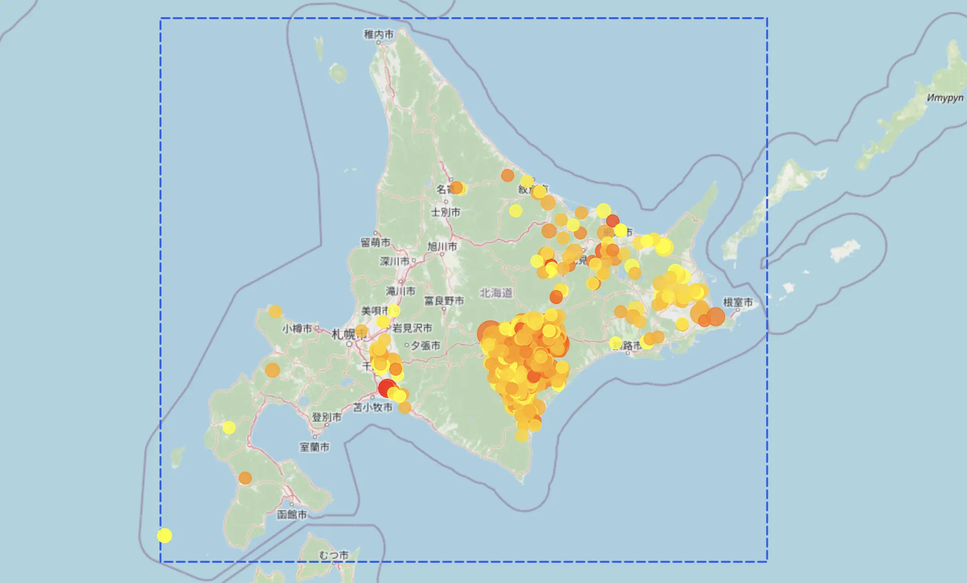
Visualizing the change scores across all of Hokkaido reveals that change points are concentrated around the Tokachi Plain. From my visual inspection, these are due to agricultural land changes.
AEF’s training targets likely influence this tendency. AEF uses not only Sentinel-2 and Landsat optical imagery but also the USDA NASS Cropland Data Layer (CDL) as one of its training targets (AEF paper Table 1). While CDL is a U.S. crop classification dataset, this training likely increases sensitivity to differences in crop types and vegetation patterns. As a result, annual vegetation changes in farmland due to crop rotation and fallow periods are readily reflected in change scores.
Below, I examine representative locations with high change scores in detail.
Tomakomai: Data Center Development Site
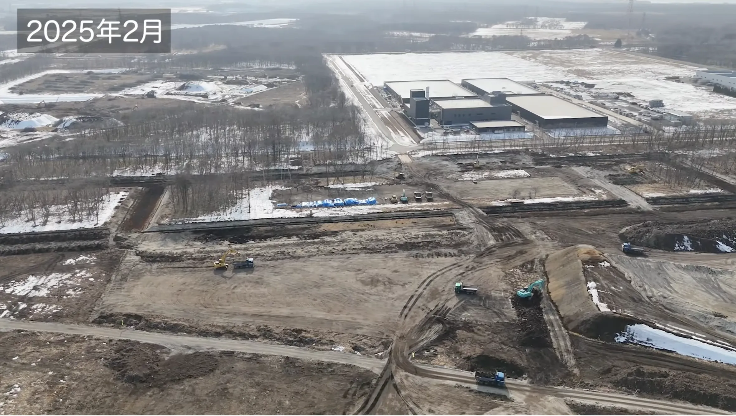
The highest change score cluster was found in the Tomakomai area. Large-scale land preparation work can be confirmed within the area enclosed by the red rectangle in the center.
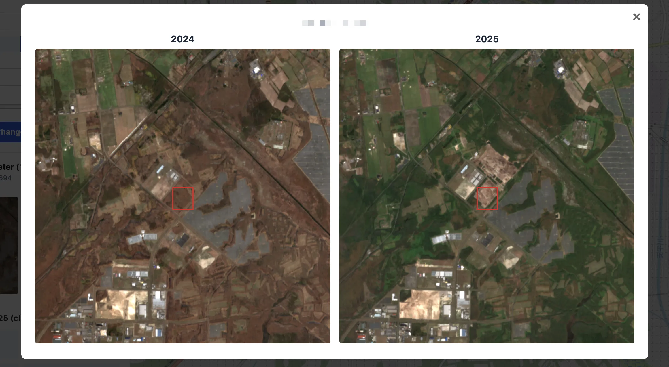
After investigating this construction, I found it to be the planned site of the “Hokkaido Tomakomai AI Data Center.” Note that due to the nature of data center facilities, the exact address is not officially disclosed, so location information is partially masked here.

Aerial footage from this article shows the before and after of the land preparation at this site. Large-scale clearing and grading of what were previously grasslands and forests enabled the Satellite Embedding to capture these changes.
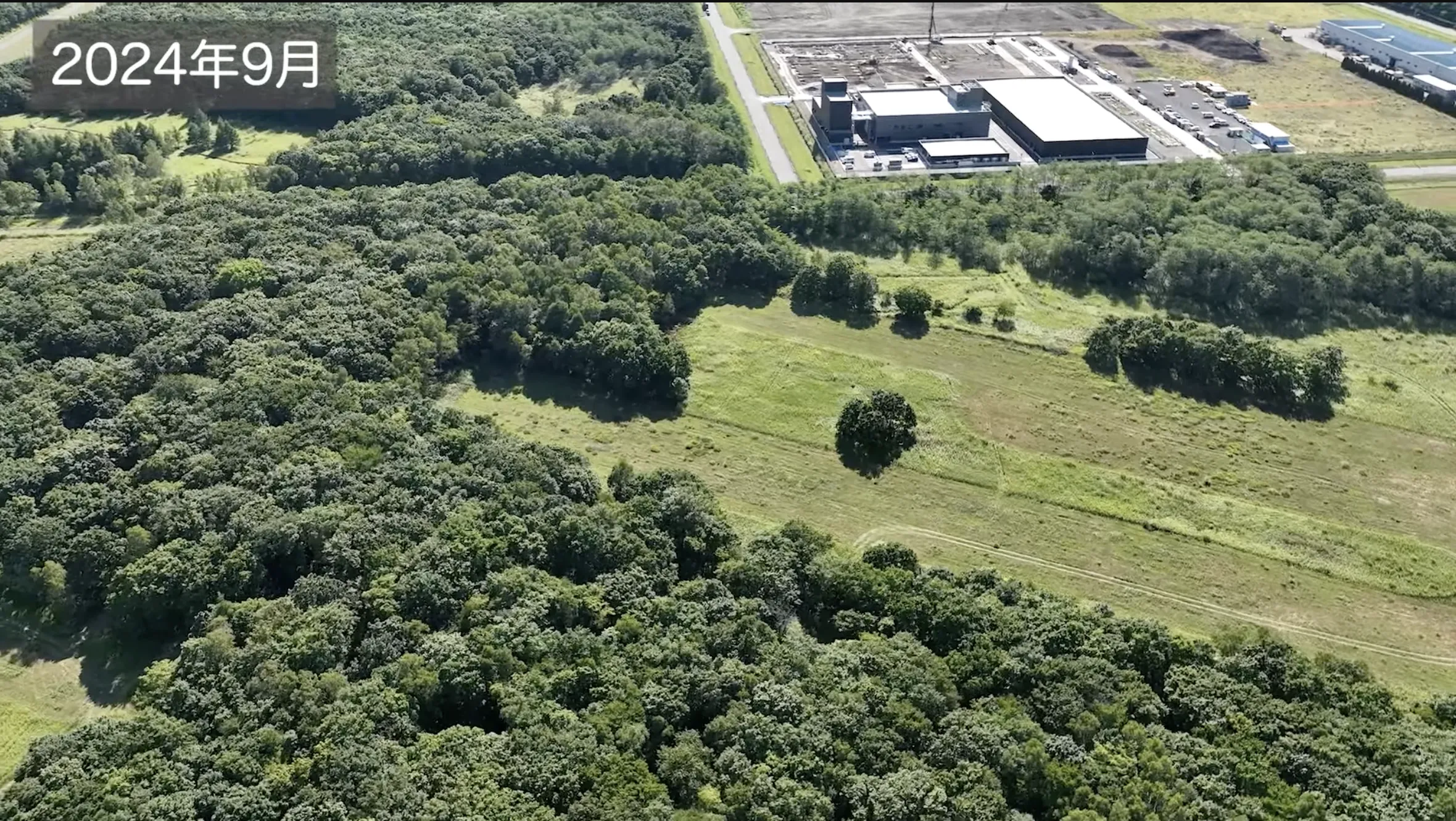 Before
 After
After
The large-scale surface changes from land preparation are clearly reflected in the embeddings, suggesting that time-series comparison of embeddings is effective for detecting development activities.
Oketo: Forest Clearing
Another case captured development activity in the forests of Oketo Town. I was unable to determine what kind of development was being carried out.
The most recent satellite imagery on Google Earth for this area is from May 22, 2024, so I could not confirm the state of construction after 2025.
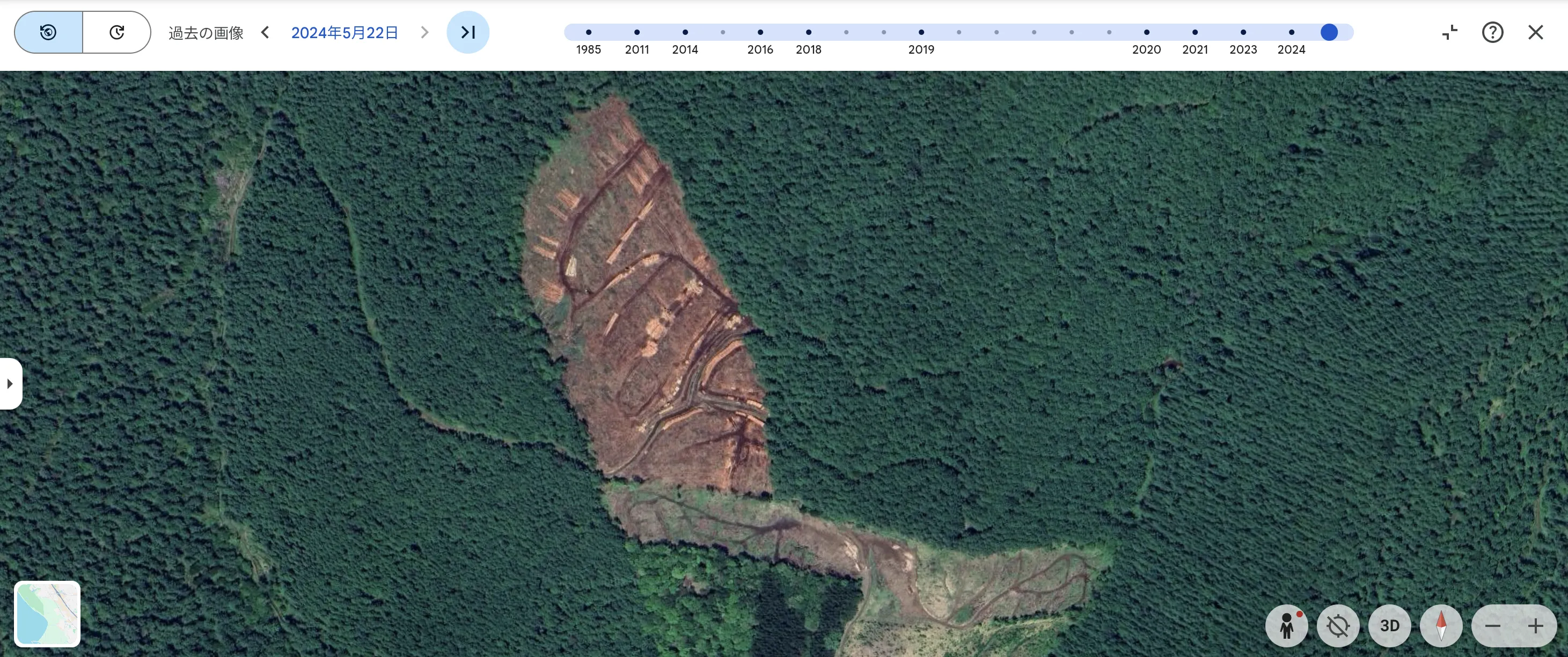
Source: Google Earth
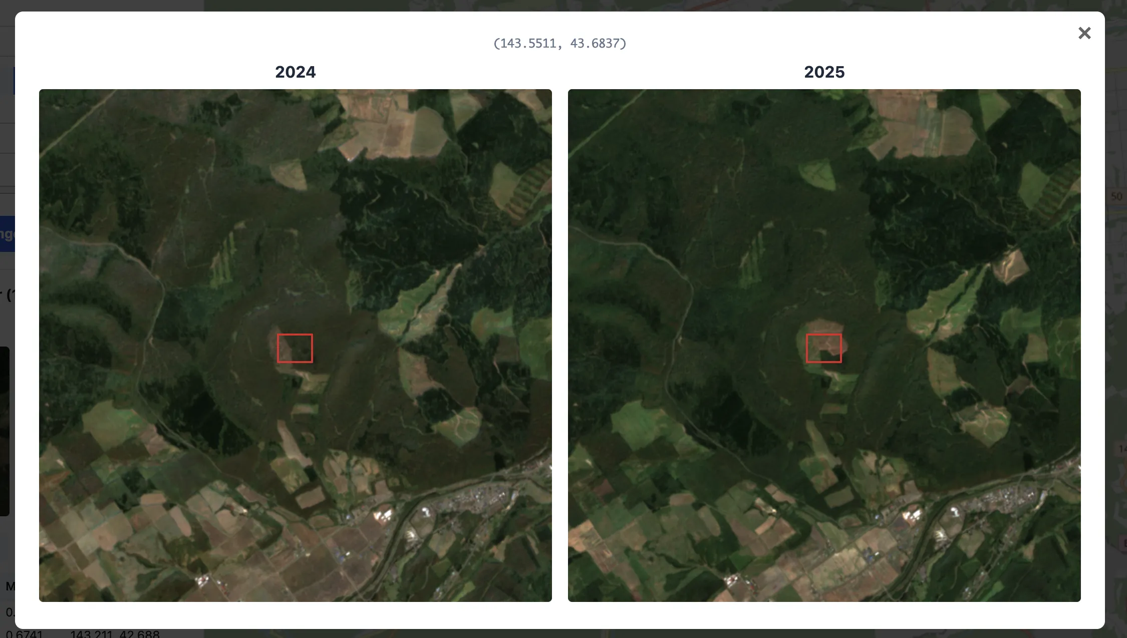
Tokachi Plain: Agricultural Land Conversion
Let me also touch on locations that appear to be farmland. The following location had the highest change score in the Tokachi Plain. Based on Google Maps and other sources, it appears that a forested section was converted to a state similar to the adjacent farmland.
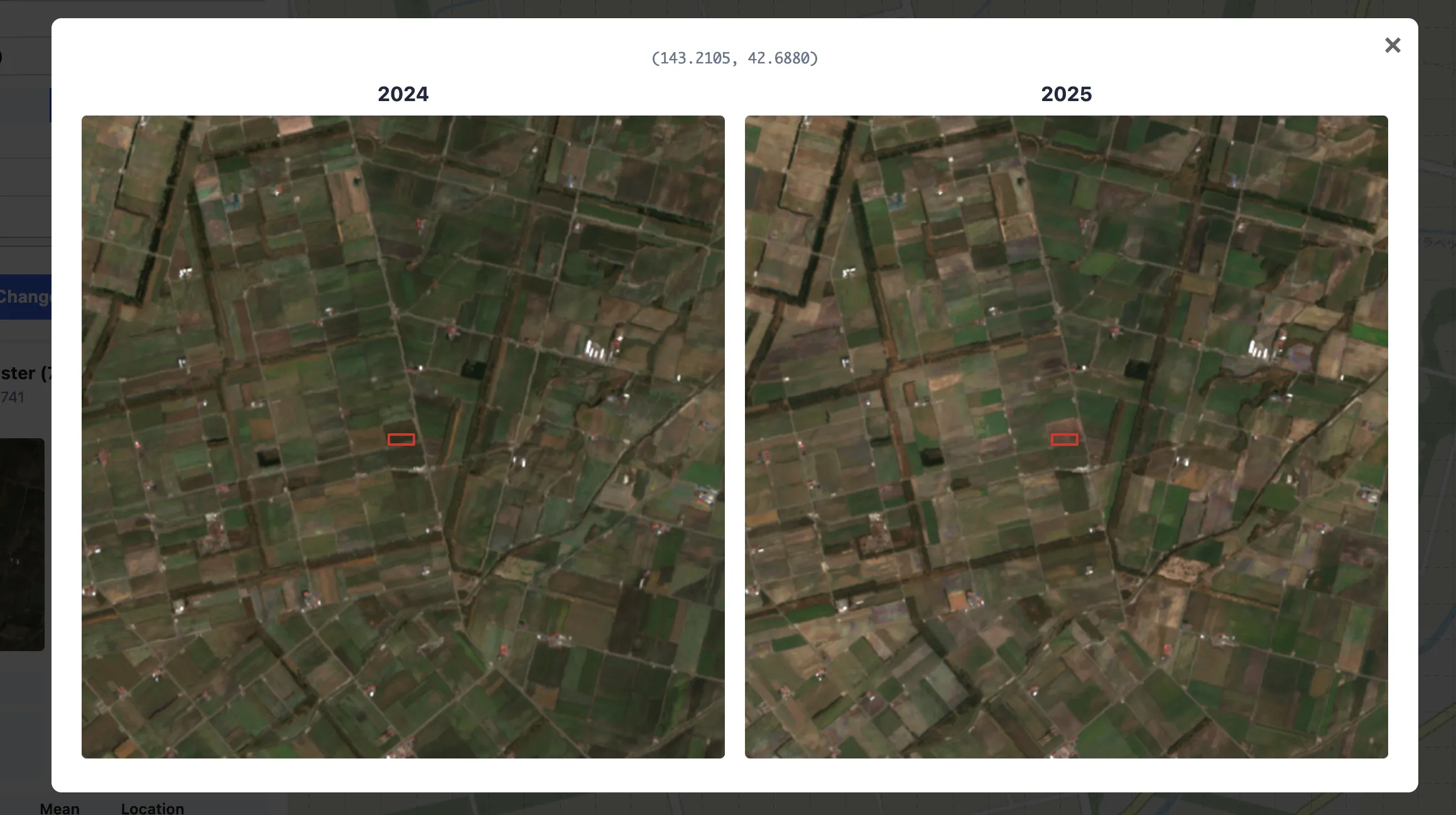
The Tokachi Plain contains numerous agricultural points with high change scores, and change scores alone cannot distinguish these from developed sites.
Conclusion
In this study, I implemented a system to detect land cover changes across approximately 15.66 million points in Hokkaido by comparing annual AlphaEarth Satellite Embeddings data. I was able to identify large-scale development activities such as data center construction sites from the top change scores, confirming that change detection leveraging the temporal consistency of the embedding space actually works.
The unsupervised change detection performance of AEF is reported in the paper’s benchmark as slightly inferior to a ViT baseline (Balanced Accuracy 71.4% vs 72.9%). While embedding-based zero-shot change detection does not match the accuracy of fine-tuned dedicated models, its ability to perform wide-area change screening without labels or additional training is a significant practical advantage.
However, this evaluation also revealed several challenges.
Challenge 1: Temporal Resolution of Annual Data
AEF’s publicly available data consists of annual composites (satellite images from an entire year combined into a single composite), making it structurally difficult to capture short-term phenomena such as floods or wildfires. The AEF paper also explicitly states that “short-lived phenomena may not be adequately captured.” For detecting such short-term changes, approaches that directly compare visible/multispectral images are more suitable.
Challenge 2: High Sensitivity to Agricultural Vegetation Changes
In this study’s results, a large number of changes originating from farmland conversion in the Tokachi Plain area were detected. Since AEF uses the USDA Cropland Data Layer as one of its training targets, it has high sensitivity to differences in crop types and vegetation patterns, resulting in farmland dominating the top change scores. Selectively extracting only structural changes such as construction and land preparation requires additional techniques such as filtering by land use type or leveraging map data.
In terms of spatial resolution as well, the current 100m grid easily captures wide-area vegetation changes like farmland but has difficulty detecting small-scale building construction or road widening. AEF provides data at intervals as fine as 10m, so using finer resolution could potentially capture such changes, but the 100x increase in data volume creates a trade-off with computational costs.